Introduction :
To the best of my knowledge, no exhaustive study of Warnsdorff’s rule for Knight’s Tour of the chessboard has been published. This paper presents the results for the work done on closed (re-entrant) solutions (tours) obtainable on a standard 8 x 8 chessboard. Since an exhaustive study was intended, no attempt has been made to resolve a tie, if it occurs along the way. Instead, all the alternative paths have been followed, without assigning priority thereto.
While conducting this study, it was noticed that strictly following the rule does not necessarily take the knight to a square with truly minimum further outlets. Some variations of the rule were hence thought of, without violating the rule in its true spirit. In doing so, some new terms such as “Corner Dash (CD)” (full or semi), “End Corner Dash (ECD)” and “Extended End Corner Dash (XCD)” have been coined and defined. All the computations have been carried out for all the 10 (Ten) unique starting points and their corresponding 53 (Fifty-three) ending points to make the tour closed.
Warnsdorff’s Rule :
Warnsdorff’s Rule[1] for Knight’s Tour states that at every step, a move should be made to a square from where there are fewest outlets to unvisited cells. This suggests that before making a move, one should work out available number of moves from each target square. All such available number of moves should be compared and the target square from where minimum further moves are available, should be chosen for making the move to that target cell.
This immediately raises a question. If there are two or more such target squares from where equal number of further moves are available and this number is minimum when compared with other remaining target squares, which target square should be chosen for the move? Many people have devised methods for resolving this “Tie”. Literature is full of rules for resolving the tie. The present work has not bothered with resolving any tie. The reason for this is already given above and will appear again later.
Previous Work Done :
The problem of Knight’s Tour of the chessboard, being at least 5 (perhaps 11 to 12) centuries old, has been widely worked on. A simple search using the Google® Search Engine easily detects several thousand significant results (web-pages). I have visited several hundred such web-pages. I have not found any work similar to the one presented here.
I have published a book[2] in which a full chapter is devoted to this subject. All the material in this paper has been extracted from the book.
Background :
A little bit of background about the present work is in order. A computer program was made in 1978 for working out Knight’s Tour solutions. It followed a so called “brute-force” method.
Moves were numbered from 1 to 8. Move number 1 was two squares to right and one square down. Going clockwise, move number 2 was two squares down and one square right, and so on, till move number 8 was two squares to right and one square up.
This scheme is shown in Figure – 1.
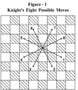
At each move, the program worked out all the available moves for the knight from where it stood. Naturally, the moves that took the knight outside the board or the moves that took the knight to an already visited square were omitted. These available moves were stored in a matrix called an Options Matrix against the move number to be made on the board. After storing all available moves from the particular square (cell), the program made the numerically highest move and deleted the move being made from the Options Matrix.
This procedure was continued, hoping that it would result in a solution. The aim was to work out all available solutions, of course, a very naïve approach. If a solution was reached, the program would store the solution and back-track by one move. Again, the numerically largest of the remaining available moves would be made and the process would continue. If at any stage the knight is stuck-up and without a further move, it would back-track by one move. Once again, the process would continue with the numerically highest move and so on.
This program did not produce even a single solution despite providing lots of CPU time on DEC-1077 mainframe computer. This is when a friend suggested using Warnsdorff’s rule. In addition to the evaluation part (of Warnsdorff’s rule) the only modification necessary in the available program was that instead of storing all the available moves at each stage, the available options were stored only when there was a tie between (among) two (or more) moves for “minimum outlets” condition. Since all the alternative paths were to be tested one-by-one, no need was felt of resolving the tie. All the options for equally minimum outlets were indeed tried out. This is the reason for labeling this work as an exhaustive study of Warnsdorff’s rule. There is one more reason for calling this as exhaustive study but that will be discussed later in appropriate context.
If there is no tie for any particular position (only a single move has minimum further outlets), then no entry is made into the Options Matrix.
As mentioned earlier, back-tracking would be invoked under two circumstances. One is when the knight is stuck-up and there is no move left. Second is when a full solution is reached. In the modified program, instead of back-tracking by one move only, it is by several moves, till the previous tie position is reached. This is easily detected by looking for a non-zero entry in the Options Matrix.
The program was modified and run in 1981. It was a pleasant surprise to find out that solutions started pouring in. Six thousand solutions were printed out on 250 pages, 24 solutions per page, with five sets of 1,200 solutions per set of 50 pages. Each set of 1,200 solutions took only between 52 and 58 seconds of CPU run time on the mainframe computer. The 6,000 solutions were studied carefully. It was found that the first 25 moves were identical in all the solutions. This meant that the solutions would be so many that it may not be feasible to record all of them. Therefore, it was decided to concentrate on getting closed solutions only. The program was once again modified to get only closed solutions. This attempt was also successful in 1981. In order to get a closed solution, the program first defines the starting point and ending point on the board. Obviously, to have a closed tour, the ending point and starting points are at a knight’s move apart. Since several sets of starting and ending points exist on the board, there are as many sets of different number of solutions in each set.
Number of Sets (Algorithms) Worked Out :
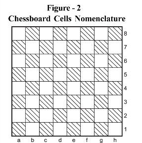
Let us first understand the co-ordinate system used. Standard notation used for recording moves of a game of chess labels the columns from left to right as “a to h”. White pieces side is at the bottom of the board, therefore, the rows are numbered from bottom to top as “1 to 8”. This system is depicted in Figure – 2.
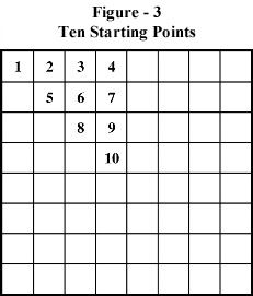
There are only 10 unique starting points on the board of 64 cells. Other 54 cells are isomorphic with these 10. These starting points are:
1) Cell a8. There are 3 more (total 4) isomorphic points on the board.
2) Cell b8. There are 7 more (total 8) isomorphic points on the board.
3) Cell c8. There are 7 more (total 8) isomorphic points on the board.
4) Cell d8. There are 7 more (total 8) isomorphic points on the board.
5) Cell b7. There are 3 more (total 4) isomorphic points on the board.
6) Cell c7. There are 7 more (total 8) isomorphic points on the board.
7) Cell d7. There are 7 more (total 8) isomorphic points on the board.
8) Cell c6. There are 3 more (total 4) isomorphic points on the board.
9) Cell d6. There are 7 more (total 8) isomorphic points on the board.
10) Cell d5. There are 3 more (total 4) isomorphic points on the board.
These starting points are shown in Figure – 3.
The corresponding ending points for a closed tour are:
1) cells c7 or b6; i.e., 2 ending points
2) cells a6, c6 or d7; i.e., 3 ending points
3) cells a7, b6, d6 or e7; i.e., 4 ending points
4) cells b7, c6, e6 or f7; i.e., 4 ending points
5) cells a5, c5, d6 or d8; i.e., 4 ending points
6) cells a8, a6, b5, d5, e6 or e8; i.e., 6 ending points
7) cells b8, b6, c5, e5, f6 or f8; i.e., 6 ending points
8) cells b8, a7, a5, b4, d4, e5, e7 or d8; i.e., 8 ending points
9) cells c8, b7, b5, c4, e4, f5, f7 or e8; i.e., 8 ending points
10) cells c7, b6, b4, c3, e3, f4, f6 or e7; i.e., 8 ending points
There are thus 53 combinations in total for all the starting and ending points, giving us 53 algorithms for working out all the solutions with Warnsdorff’s rule.
Working of the Computer Program :
With the background as above, we are ready to understand the working of the program and how all the options from Warnsdorff’s rule are tried out one after another. We will generate the first solution along with its options matrix. The starting point selected is the top left corner of the board, the cell “a8”. This gets the number 1. From here, we start evaluating each move before actually making any move. From square marked 1, we have two moves available. Move type 1 takes us to cell “c7” and move type 2 takes us to cell “b6”. Since we are aiming to make the tour closed, the cell “c7″is arbitrarily reserved for move number 64. Hence, the only target cell now left is b6. We write the number 2 in this cell, i.e., move the knight to this square b6.
From the cell marked 2, we have five moves available. Move type 1 takes us to cell “d5”, type 2 takes us to cell “c4”, type 3 takes us to cell “a4”, type 7 takes us to cell “c8” and type 8 takes us to cell “d7”. From d5 and c4, there are 7 outlets available. From d7, there are 5 outlets. From a4 and c8, there are 3 outlets. The minimum number of outlets is 3 and these are from two target cells, a4 and c8. There is thus a tie for this move. Any one move can be chosen, reserving the other for later evaluation. As per the program logic, the numerically higher move (type 7) is chosen, taking us to c8. At the same time, Options Matrix stores the information that from cell numbered 2 move type 3 was also having minimum outlets. This is achieved by storing the number 3 at location MO(2,1). Here, MO is the options matrix with DIMENSION (64,8).
Thus, we write the number 3 in the cell c8 and proceed further. The further working is continued in similar manner till we reach the cell a5 at move number 20. From here, there are three target cells by move types 1, 2 and 8; reaching c4, b3 and c6 respectively. When we evaluate the number of outlets from each of these target cells, we find that from each target cell, there are exactly 4 outlets. Thus, there is a triple tie. As before, per program logic, we select the last direction (8) and move to cell c6 and write the number 21 in that cell. Now, we have here two more target cells to be remembered within the Options Matrix, having equal number of outlets to the selected option. This is done by storing (move type) number 1 at MO(20,1) and storing (move type) number 2 at MO(20,2).
Further working is not discussed in detail. By proceeding further as per above algorithm, we complete the tour as per Figure 4. This is the first solution obtained with this method.
There was no need to use back tracking of moves even once. While generating the solution, there are further entries in the options matrix MO whenever there are two or more target cells with equal number of minimum outlets. Having obtained the first solution as above, now let us see how we can generate more solutions from the first one. First, let us review the nonzero entries in the options matrix MO. These are at (2,1), (20,1), (20,2), (41,1), (41,2), (43,1), (47,1), (48,1) and (49,1) being the last nonzero entry. Hence, we come back to the cell e6 marked 49, erasing the numbers 50 through 64 working manually, or storing 0 (zero, signifying that the square is available [unvisited] for the knight) into those locations when the computer program back tracks to the cell e6 marked 49. At this point, we see that MO(49,1) had the value 2. So, we make move type 2 and write number 50 in cell f4. At the same time, we set the value of location MO(49,1) to 0 (zero) because we have now used up the option. The further working is normal upto the solution obtained in Figure – 5 as the second solution by this method. Here, at move 54, there is a tie and a nonzero entry MO(54,1) = 5 gets generated.


Corner Dash (CD) Concept :
It is quite obvious that in order to complete the tour, the four corners also have to be covered in the tour. There is a peculiarity here. Each corner can be visited only from one of the two approach cells. If the knight lands on one of them, it is imperative that the knight immediately visits the corner and then comes out from the other approach cell. This, in a way, restricts the choices available at the approach cells.
For the starting point a8 and ending point c7 discussed above for generating first few solutions, consider the position when the knight reaches the cell marked number 6, as depicted in Figure – 6.
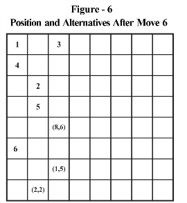 As usual, we mark the number of further moves from the target cells c2, b1 and c4. From cell c2, there are 5 possible moves. From cell c4, there are 6 possible moves. From cell b1, there are only 2 further moves. As per Warnsdorffs rule, cell b1 gets selected and quite properly so.
However, the cell c2 is one of the two cells for approaching the corner at cell a1, the other being the cell b3. Hence, availability of 5 moves from c2 is illusory, there being an urgent need to visit the corner at a1. In reality, there is only 1 move (and not 5 moves) available from c2. Thus, there is a strong case for jumping from a3 to c2 rather than from a3 to b1 (This is not a violation of Warnsdorffs rule but we are applying it in its spirit rather than applying it by its word). What if we over-ride our usual criterion for this move only and force the knight to jump to cell c2 instead of to b1? From c2, the knight can visit the corner at a1 (even as per Warnsdorff’s rule and the program logic), come out to cell b3 and continue the tour as per Warnsdorffs rule. This forced jump that temporarily overrides the normal program logic has been termed as making a Dash to the corner or simply “Corner Dash (CD)”.
This over-riding of normal program logic, or corner dash, can be done at all four corners, near cells a1, a8, h1 and h8. However, in the first set, the corner at cell a8 is not available to us for corner dash because we have made it the starting point for our tour. With three corners available for corner dash, total eight algorithms can be created as follows –
1) Algorithm with no corner dash (original program).
2) Algorithm with only one corner dash
a) Top Right corner (cell h8) dash
b) Bottom Left corner (cell a1) dash
c) Bottom Right corner (cell h1) dash
3) Algorithm with two corners dash
a) Except Bottom Right, other corners (cells a1 and h8) dash
b) Except Bottom Left, other corners (cells h1 and h8) dash
c) Except Top Right, other corners (cells a1 and h1) dash
4) Algorithm with all the three corners (cells a1, h1 and h8) dash
Now we have total 8 algorithms instead of only 1 (additional 7). We stand to get many more different solutions for the tour. When we take the starting point away from the corner, e.g., b8 or c8, all the four corners are available for corner dash. We then get following 16 algorithms instead of just 1 (additional 15) –
1) Algorithm with no corner dash (original program).
2) Algorithm with only one corner dash
a) Top Left corner (cell a8) dash
b) Top Right corner (cell h8) dash
c) Bottom Left corner (cell a1) dash
d) Bottom Right corner (cell h1) dash
3) Algorithm with two corners dash
a) Top Left and Top Right corners (cells a8 and h8) dash
b) Top Left and Bottom Left corners (cells a8 and a1) dash
c) Top Left and Bottom Right corners (cells a8 and h1) dash
d) Top Right and Bottom Left corners (cells a1 and h8) dash
e) Top Right and Bottom Right corners (cells h1 and h8) dash
f) Bottom Left and Bottom Right corners (cells a1 and h1) dash
4) Algorithm with three corners dash
a) Top Left, Top Right and Bottom Left corners (cells a8, h8 and a1) dash
b) Top Left, Top Right and Bottom Right corners (cells a8, h8 and h1) dash
c) Top Left, Bottom Left and Bottom Right corners (cells a8, a1 and h1) dash
d) Top Right, Bottom Left and Bottom Right corners (cells h8, a1 and h1) dash
5) Algorithm with all the four corners dash
When we apply Corner Dash concept to all the 53 combinations of starting and ending points, we get total of 736 algorithms to work with. The computer program was modified for each run and solutions were worked out. The total number of solutions jumped to 5,201,841.
Semi Corner Dash Concept :
In the example for explaining the concept of corner dash (Figure – 6), we saw how the move evaluation process as per Warnsdorff’s rule could be modified for selecting the cell c2 for the move instead of moving the knight to b1. Remembering that there are two approach cells for any corner, depending upon how the tour has progressed, it could have been the square b3 where the selection process could have to be modified. Therefore, the corner dash logic inside the computer program is such that if the target square for the knight is either b3 or c2, then consider that it has only one further exit and select that target square for the next move.
Now, suppose that we wish to allow the corner dash only if the square involved is b3 and not if it is c2. Alternatively, we wish to allow the corner dash only if the square involved is c2 and not if it is b3. In these cases, each of the two conditions is termed as a “Semi Corner Dash” because it involves only one out of two approach cells for the corner.
What is the advantage or sense in this semi corner dash? Surprisingly, many times entirely different solutions (tours) are found by employing this idea. The number of solutions is also quite large. If we label one approach cell as A and the other as B, for a single corner, we get 3 sets of solutions. We may call them set A, set B or set C where, C means either A or B, i.e., “full” corner dash (the one we learned before semi corner dash). Since the case C has been already included in the 736 algorithms, we have two extra sets of solutions, A and B.
For two corners dash, there will be total 32 = 9 sets out of which one set will be with both full corner dashes. We then get 8 extra sets of solutions. Going further, for three corners dash, 33 = 27 and for four corners dash, 34 = 81 sets are present. In both these cases there is one set with all full corner dash, leaving us with 26 and 80 extra sets of solutions respectively. For the 736 algorithms with 0, 1, 2, 3 or 4 corners dashes, there are total 10,144 semi corner dash algorithms. All those runs were done to obtain 40,639,273 extra solutions. Adding the solutions for the 736 algorithms, the total solutions obtained were 45,841,114. This is 46.3 times the number of solutions obtained by strictly following Warnsdorff’s rule by word. Following the rule in spirit has paid huge dividends!
The details about the number of solutions obtained from each algorithm, with full or semi corner dash, are given in the Table AlgoMain by following the link.
Concept of End Corner Dash (ECD) :
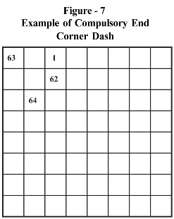
Observe set 3(b), i.e., starting point c8 (getting the number 1) and ending at b6 (getting the number 64). The cell b6 happens to be the access cell for the corner at a8. Therefore, the tour cannot be completed unless the cell a8 has number 63 and naturally the other access cell c7 must be 62. The corner is hence visited in the end. This is hence called end corner dash (ECD). In this case, there is no option but to cover the corner in the end only. Hence, such an end dash is called compulsory. Starting point and last few moves of this compulsory end corner dash are shown in Figure – 7.
One must distinguish this from a case when the end dash is optional. For example take the set 2(a) with starting point at b8 and ending point at a6. Here the normal full and semi corner dashes exist and algorithms numbered 17 to 32 have been included already. An interesting observation is that the ending cell a6 is just one move away from the corner access cell c7. Why not force the program to visit the a8 corner in the end only and not during the course of normal tour? The cells b6, a8, c7 and a6 will then get the numbers 61, 62, 63 and 64 respectively. This is the end corner dash. This end dash is of optional (not compulsory) type. Starting point and last few moves of this optional end corner dash are shown in Figure – 8.

Once again, the justification for making this kind of variation in knight’s tour is for getting more solutions! All the 53 combinations of starting and ending points were carefully checked for possibility of ECD. Total 32 such ECD were noted.
As one corner is being reserved for ECD, only 3 corners are available for our usual full and semi corners dash. That gives total 8 algorithms with 0, 1, 2 or 3 full corners dashes and 56 semi corner dashes. Total of 256 algorithms for full dashes and 1,792 algorithms for semi dashes are obtained. The program was suitably modified and run 2,048 (256 + 1,792) times. For the 256 algorithms, 570,079 solutions and for 1,792 semi corner dashes, 2,366,427 solutions (tours) were obtained.
The details about the number of solutions obtained from each algorithm, with full or semi corner dash, are given in the Table AlgoECD by following the link.

